Opening the black box

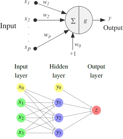
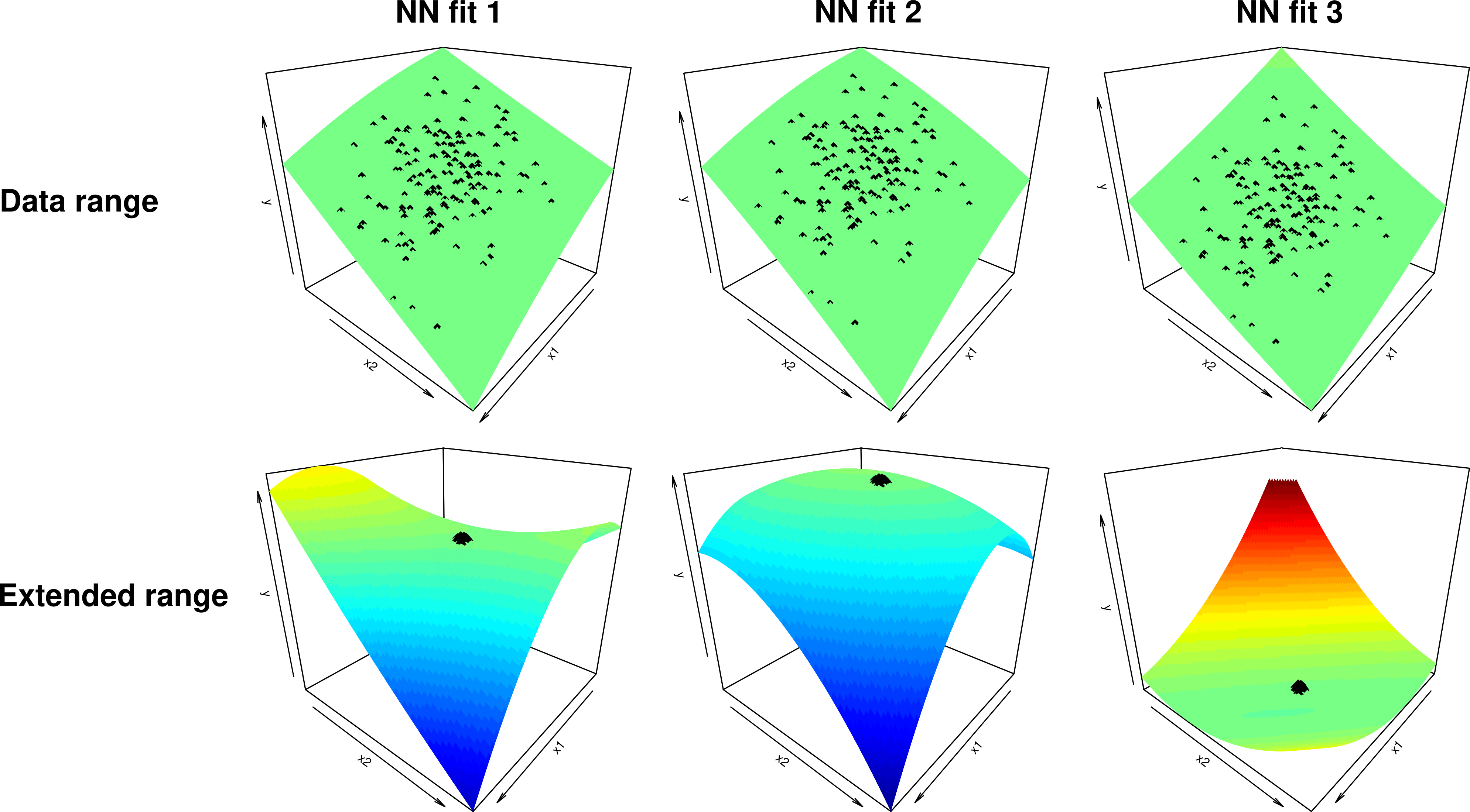
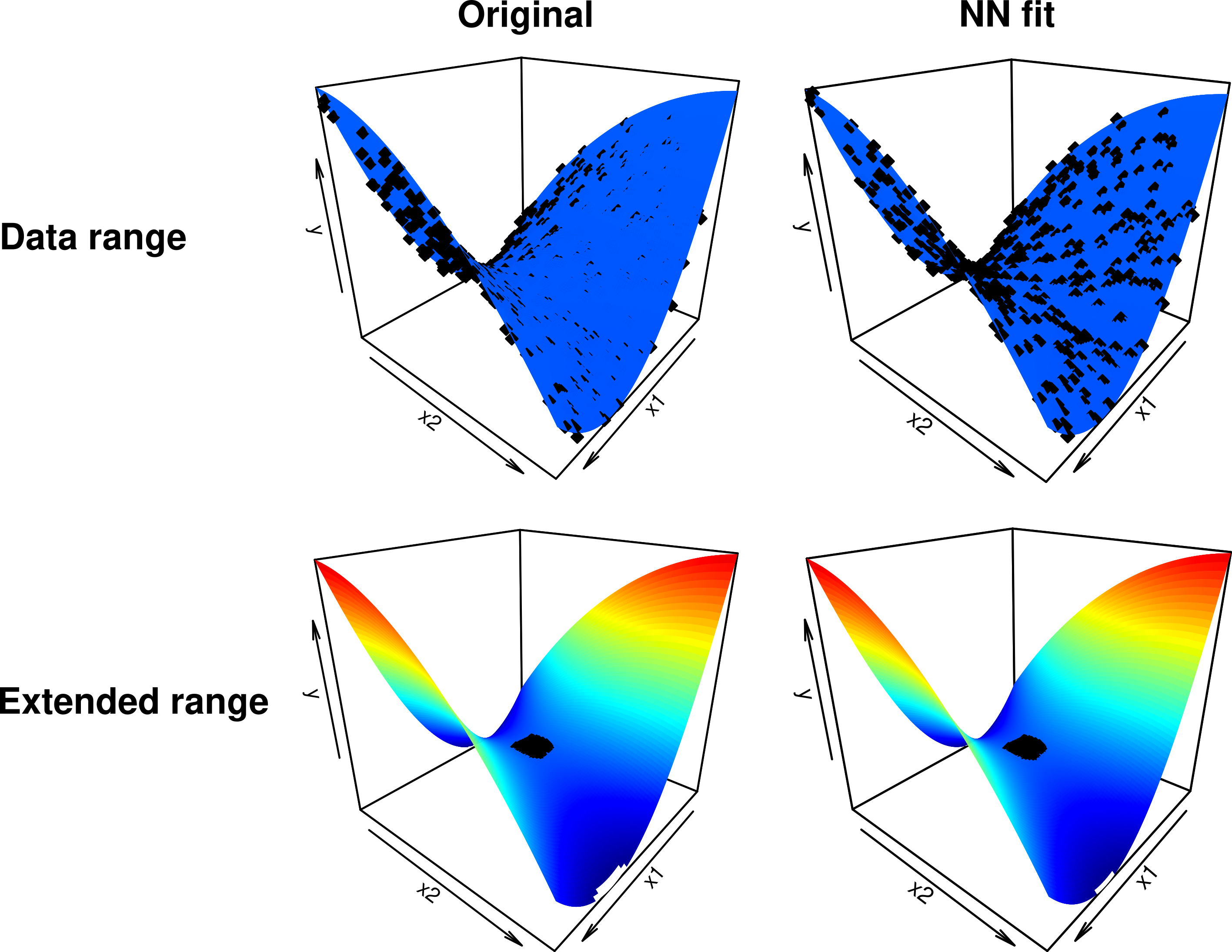
class: center, middle, inverse, title-slide

.title[
# Opening the black box
]
.subtitle[
## From Neural Nets to Polynomials and beyond
]
.author[
### Iñaki Úcar | Postdoctoral Fellow @ IBiDat
]
.date[
### June 2, 2022
]

---

# Context

.research-left-column[

## Statistical software

- **R project** contributor since 2015
  - 9 packages on CRAN
- Maintainer of **r-simmer** DES
  - Published in the JSS
- Co-maintainer of **r-quantities**
  - Published in the R Journal
  - Funded by the R-Consortium
- Member of the **Rcpp Core** team
- Co-founder of **ROpenSpain**

]

![:tail](Technology transfer)

.research-right-column[

## Social applications

- Socioeconomic status
- Inequality
- Mobility
- ...

#### Projects:
- **CONCIERGE-CM-UC3M** (co-PI)
 - with Marga Torre Dept. Social Sciences, UC3M
- **StatPhys4Cities**
 - with Esteban Moro Dept. Mathematics, UC3M MIT Media Lab

]

.research-overlay[.research-center-column[

## Interpretability of NN

- From business needs
- Started as exploratory TFMs
- then Pablo Morala's thesis co-supervision
 - Rosa E. Lillo
 - J. Alexandra Cifuentes

#### Outline:
- Initial work (paper)
  - [10.1016/j.neunet.2021.04.036](https://doi.org/10.1016/j.neunet.2021.04.036)
- Current status (preprint)
  - [10.48550/arXiv.2112.11397](https://doi.org/10.48550/arXiv.2112.11397)
- Open challenges, vision, impact

]]

---
class: inverse, center, middle

# Interpretability of .emph[Neural Networks] via .emph[Polynomials]

---
class: base24

# Introduction

.left-column[
### Motivation
]

.right-column[
Machine learning (ML) is a **growing trend** in many organisations 
Neural Networks (NNs) and Deep Learning (DL) are achieving a great success
]

.right-column-append[
**Drivers:**
- Big Data (both structured and non-structured)
- Cloud Computing
- Prediction performance
]

.right-column-append[
**Blockers:**
- Fairness
- Explainability, interpretability
- Regulations
]

---
class: base24

# Introduction

.left-column[
### Motivation
### Seminal paper
]

.right-column[
![:bqh](Preprint)
> Cheng, X., Khomtchouk, B., Matloff, N., Mohanty, P. (2019).
> _Polynomial Regression As an Alternative to Neural Nets._
> _arXiv_ [cs.LG, stat.ML].
> DOI: [10.48550/arXiv.1806.06850](https://doi.org/10.48550/arXiv.1806.06850)

Presents the following ideas:
- NNs.emph[*] are a form of Polynomial Regression (PR).
- The **degree** of the polynomial increases with each hidden layer.
- PR properties can be used to study and even **solve NN problems**.
- **Experimental results**: PR as good as NNs in the studied datasets.
- Using PR instead of NNs: **R package {polyreg}**.

.footnote[.emph[*] Specifically, fully-connected feed-forward NN, AKA multilayer perceptrons (MLPs).]
]

---
class: base24

# Introduction

.left-column[
### Motivation
### Seminal paper
### Main idea
]

.right-column[
**Transform a trained NN into an .emph[equivalent] polynomial**

.pull-left[
Objectives:
- Explicit model
- Reduced number of parameters
- Interpretability of coefficients
- ...
- Study NN properties
- Inform NN dimensioning
- ...
]
.pull-right[
![](img/nn.svg)
]
]

---
class: base24

# Framework

.left-column[
### Initial work
]

.right-column[
![:bqh](Article)
> Morala, P., Cifuentes, J. A., Lillo, R. E., **Ucar, I.** (2021a).
> _Towards a framework to inform neural network modelling via polynomial regression._
> _Neural Networks_, 142, 57–72.
> DOI: [10.1016/j.neunet.2021.04.036](https://doi.org/10.1016/j.neunet.2021.04.036)

Main merits:

- Find an **explicit expression** to build a polynomial from the .emph[weights]
  of a trained MLP, using a .emph[Taylor expansion] of the activation function
  - Limited to a single hidden layer and linear output
  - Weights need to be constrained for the expansion to remain valid
- Validated through a **simulation study**
]

---
class: base24

# Framework

.left-column[
### Initial work
### Notation
]

.right-column[
Polynomial of degree `$k$` in `$p$` variables:
`$$z = \beta_{0} + \underbrace{\beta_{1} x_{1} + \dots + \beta_{p}x_{p}}_{1\mbox{-order interactions}} +\dots + \underbrace{\beta_{1 p\dots p}x_1x_p^{k-1} + \dots + \beta_{p\dots p}x_p^{k}}_{k\mbox{-order interactions}}$$`
]

.right-column-append[
.pull-left[
Hidden layer, neuron `$j$`:
`$$y_j = g(u_j) = g\left(\sum_{i=0}^p w_{ij} x_{i} \right)$$`
Final output:
`$$z=\sum_{j=0}^{h_1} v_{j} y_{j} = \sum_{j=0}^{h_1} v_{j} g\left(\sum_{i=0}^p w_{ij} x_{i} \right)$$`
]

.pull-right[
![:scale 70%](img/shlnn.png)
]
]

---
class: base24

# Framework

.left-column[
### Initial work
### Notation
### Tools
]

.right-column[
Taylor expansion of the activation function `$g$`:
`$$y_j=g\left(\sum_{i=0}^pw_{ij}x_i\right)=\sum_{n=0}^{\infty}\frac{g^{(n)}(a)}{n!}{\color{blue}\left(\sum_{i=0}^pw_{ij}x_i-a\right)^n}$$`

Binomial theorem:
`$${\color{blue}\left(\sum_{i=0}^p w_{ij}x_{i}-a\right)^n} = \sum_{k=0}^n \binom{n}{k}(-a)^{n-k}{\color{magenta}\left(\sum_{i=0}^pw_{ij}x_i\right)^k}$$`

Multinomial theorem:
`$${\color{magenta}\left(\sum_{i=0}^p w_{ij}x_{i}\right)^k} = \sum_{m_{0}+\cdots+m_{p}=k}{\binom{k}{m_{0}, \dots, m_{p}}} (w_{0j}x_{0})^{m_{0}} \cdots (w_{pj}x_{p})^{m_{p}}$$`
]

---
class: base24

# Framework

.left-column[
### Initial work
### Notation
### Tools
### Coefficients
]

.right-column[
Output expanded at `$a=0$`, truncated at degree `$q$`:
`$$z\approx v_0+\sum_{j=1}^{h_1}v_j\sum_{n=0}^{q}\dfrac{g^{(n)}(0)}{n!}\left[\sum_{m_{0}+\cdots+m_{p}=n}{\binom{n}{m_{0}, \dots, m_{p}}} (w_{0j}x_{0})^{m_{0}} \cdots (w_{pj}x_{p})^{m_{p}}\right]$$`

**Intercept:**
`$$\beta_0=v_0+\sum_{j=1}^{h_1}v_j\left(\sum_{n=0}^{q}\frac{g^{(n)}(0)}{n!}w_{0j}^{n}\right)$$`

**Interactions of order `$T$`:**
`$$\beta_{t_1t_2\dots t_T}=\sum_{j=1}^{h_1}v_j\left(\sum_{n=T}^{q}\frac{g^{(n)}(0)}{(n-T)!\cdot m_1!\cdots m_p!} w_{0j}^{n-T}w_{1j}^{m_1}\dots w_{pj}^{m_p}\right)$$`
]

---
class: base24

# Framework

.left-column[
### Initial work
### Notation
### Tools
### Coefficients
### `$g$` expansion
]

.right-column[
.pull-left-mod[
Example: **softplus**
`$$g(x)=\ln\left(1+e^x\right)$$`

Legend:
- Real function
- .red[Taylor expansion], order `$q$`
- .blue[Error] (difference)
]

.pull-right-mod[
![](img/Taylor_expansion_softplus.svg)
]
]

---
class: base24

# Simulation study

.left-column[
### Procedure
]

.right-column[
![:scale 88%](img/experimental_framework_diagram.svg)
]

---
class: base24

# Simulation study

.left-column[
### Procedure
### Results I
]

.right-column[
.pull-left-mod[
(1) Good case 
(2) Bad case

(A) Response vs. Predicted NN 
(B) Predicted NN vs. Polynomial 
(C) Expansion validity region + &emsp;&ensp;dist. of activations `$u_j$`
]

.pull-right-mod[
![](img/Performance_Examples_Together.svg)
]
]

---
class: base24

# Simulation study

.left-column[
### Procedure
### Results I
### Performance I
]

.right-column[
.pull-left-mod[
- 500 MSE simulations
- Data scaled to `$[-1, 1]$`
]

.pull-right-mod[
![](img/MSEBoxplots-1,1.svg)
]
]

---
class: base24

# Simulation study

.left-column[
### Procedure
### Results I
### Performance I
### Surfaces I
]

.right-column[
![](img/surfaces-1.png)
]

---
class: base24

# Framework

.left-column[
### Initial work
### Notation
### Tools
### Coefficients
### `$g$` expansion
### Constraints
]

.right-column[
**Limited region** where Taylor expansion is accurate
]

.right-column-append[
- Impose an `$\ell_1$`-norm equal to one for the hidden layer weights:
  `$$\left\lvert \left\lvert \vec{w}_{j} \right\rvert \right\rvert_1 = \sum_{i=0}^p \left\lvert w_{ij} \right\rvert = 1$$`
- Then the **activations `$u_j$` are also constrained** by 1 in absolute value:
  `$$\lvert u_j \rvert = \left\lvert \sum_{i=0}^p w_{ij} x_{i} \right\rvert \leq  \sum_{i=0}^p \left\lvert w_{ij} x_{i} \right\rvert \leq  \sum_{i=0}^p \left\lvert w_{ij} \right\rvert = \left\lvert \left\lvert \vec{w}_{j} \right\rvert \right\rvert_1 = 1,$$`
where `$\left\lvert x_i\right\rvert \leq 1$` because of the `$[-1,1]$` scaling. Therefore, `$\left\lvert u_j\right\rvert \leq 1$`
]

---
class: base24

# Simulation study

.left-column[
### Procedure
### Results I
### Performance I
### Surfaces I
### Results II
]

.right-column[
![:scale 77%](img/Performance_example_bounded_weights.svg)
]

---
class: base24

# Simulation study

.left-column[
### Procedure
### Results I
### Performance I
### Surfaces I
### Results II
### Performance II
]

.right-column[
![:scale 90%](img/Boxplots_bounded_weights.svg)
]

---
class: base24

# Simulation study

.left-column[
### Procedure
### Results I
### Performance I
### Surfaces I
### Results II
### Performance II
### Surfaces II
]

.right-column[
![:scale 72%](img/surfaces-2.png)
]

---
class: base24

# Framework

.left-column[
### Current status
]

.right-column[
![:bqh](Preprint)
> Morala, P., Cifuentes, J. A., Lillo, R. E., **Ucar, I.** (2021b).
> _NN2Poly: A polynomial representation for deep feed-forward artificial neural networks._
> _arXiv_ [stat.ML, cs.LG].
> DOI: [10.48550/arXiv.2112.11397](https://doi.org/10.48550/arXiv.2112.11397)

Main merits:
- **Extend** previous work to MLPs with an .emph[arbitrary number] of hidden layers
- **Extend** previous work to classification problems

Underway:
- Improve notation
- Model the error
]

---
class: base24

# Framework

.left-column[
### Current status
### Notation
]

.right-column[
Consider a MLP with `$L-1$` hidden layers (0: input; `$L$`: output)

Output at layer `$l$`, neuron `$j$`:
`$$\prescript{(l)}{}{y}_j = \prescript{(l)}{}{g}\left(\prescript{(l)}{}{u}_j\right) = \prescript{(l)}{}{g}\left(\sum_{i=0}^{h_{l-1}}\prescript{(l)}{}{w}_{ij}\prescript{(l)}{}{x}_i\right)$$`

Polynomial at layer `$l$`, neuron `$j$` of order `$Q_{l-1}$` in `$p$` variables:
`$$\prescript{(l)}{}{P}_j\left(p,Q_{l-1}\right) = \sum_{\vec{t} \in \mathcal{T}(p,Q_{l-1})} \prescript{(l)}{}{B}_{j,\vec{t}}$$`
where `$B_{\vec{t}} = \beta_{\vec{t}} \cdot x_{t_1}\dots x_{t_T}$` and `$\mathcal{T}(p,Q_{l-1})$` is the set of all possible interactions
]

---
class: base24

# Framework

.left-column[
### Current status
### Notation
### Algorithm
]

.right-column[
Using the first contribution, obtain the activation `$\prescript{(2)}{}{u}_j \approx \prescript{(2)}{\mathrm{in}}{P}_j\left(p,Q_{1}\right)$`
]

.right-column-append[
For `$l=2\dots L-1$`:
- Apply the Taylor expansion of the non-linearity `$\prescript{(l)}{}{g}$`:
  `$$\prescript{(l)}{}{y}_j \approx \prescript{(l)}{}{g}\left(\prescript{(l)}{}{u}_j\right) \approx \prescript{(l)}{\mathrm{out}}{P}_j\left(p,Q_{l}\right)$$`
]

.right-column-append[
- Obtain the activation `$\prescript{(l+1)}{}{u}_j$` for each neuron `$j$` at layer `$l+1$`:
  `$$\prescript{(l+1)}{}{u}_j \approx \prescript{(l+1)}{\mathrm{in}}{P}_j\left(p,Q_{l}\right)$$`
]

.right-column-append[
If it's a classification problem, apply the expansion of the non-linearity `$\prescript{(L)}{}{g}$`
]

---
class: base24

# Framework

.left-column[
### Current status
### Notation
### Algorithm
### Coefficients
]

.right-column[
**Interactions** at layer `$l$`, neuron `$j$` after including `$\prescript{(l)}{}{g}$` effect:
`$$\prescript{(l)}{\mathrm{out}}{{\beta}}_{j,\vec{t}} = 
 \sum_{n=0}^{q_{l}}\dfrac{\prescript{(l)}{}{g}^{(n)}(0)}{n!}
 \sum_{ \vec{m} \in \pi(\vec{t},l,n)}
 \left(\begin{array}{c} n \\ \vec{m}_{p,Q_{l-1}} \end{array}\right)\prod_{k=1}^{M_{p,Q_{l-1}}} \prescript{(l)}{\mathrm{in}}{\beta}_{j,k}^{m_{k}}$$`
where `$\pi(\vec{t},l,n)$` is .emph[the set of all possible partitions] for a given combination of variables `$\vec{t}$`, layer `$l$` and order `$n$`
 
**Interactions** for the linear case at layer `$l+1$`, neuron `$j$`: 
(e.g., when `$l+1=L$` for the only output neuron in regression problems)
`$$\prescript{(l+1)}{\mathrm{in}}{\beta}_{j,\vec{t}} = \sum_{i=0}^{h_{l}}\prescript{(l+1)}{}{w}_{ij} \cdot \prescript{(l)}{\mathrm{out}}{\beta}_{i,\vec{t}}$$`
]

---
class: base24

# Simulation study

.left-column[
### Procedure
### Results I
### Performance I
### Surfaces I
### Results II
### Performance II
### Surfaces II
### Results III
]

.right-column[

Example with **several layers**:

- Output polynomial matches NN predictions
- The distribution of activations `$\prescript{(l)}{}{u}_j$` is constrained at every hidden layer

.pull-left[
![:scale 100%](img/fig_performance_l1.svg)
]
.pull-right[
![:scale 100%](img/fig_taylor_layers_l1.svg)
]
]

---
class: base24

# Summary

.left-column[
### Conclusions
]

.right-column[
**Main contribution**: An .emph[explicit formula] to obtain an .emph[equivalent] polynomial from the weights of a trained MLP
- The polynomial predicts as well (or as bad) as the NN
- **Main advantage**: .emph[interactions] vs. simple feature importance
]

.right-column-append[
The method provides polynomials **at each layer and neuron**, so it can be used to represent parts of a network by taking only the weights of a section and treating them like a smaller new NN
]

.right-column-append[
This framework can be used to **interpret** NNs predictions, **study** their properties and explore how to **tune** their hyperparameters
- And much more, e.g. explore how the training evolves
]

---
class: base24

# Summary

.left-column[
### Conclusions
### Open challenges
]

.right-column[
**Computationally expensive** combinatorial problem
- Equivalent to finding the partitions of the multiset `$\vec t$`
- Only one algorithm, by none other than... .emph[Donald Knuth]! in the 1980s
]

.right-column-append[
Explicit formula for the **error**, CIs for the coefficients
]

.right-column-append[
Applications to **real datasets**
- Is the polynomial representation unique?
]

.right-column-append[
Extensions to **other architectures** and non-tabular data
]

---
class: inverse, center, middle

# Wrap-up

---

# Vision and impact

.research-center-column[

## Interpretability of NN

- **NN2Poly** framework
- Error estimation
- Inform NN design
- Sensitivity analysis
- Extensions to other architectures
- ...

]

![:tail wide](Society, administration, businesses...)
![:arrow up, 570px, 500px](Actual needs)

.research-left-column[

## Statistical software

- Computational issues
- Software packages

]

![:arrow left, 430px, 400px]()
![:arrow down, 166px, 500px](Technology transfer)

.research-right-column[

## Social applications

- **StatPhys4Cities**
  - interpretable mobility models
- ...

]

![:arrow right, 849px, 400px]()
![:arrow down, 930px, 500px](Knowledge, policies)

---
class: inverse, center, middle

# Thanks! Questions?

Slides created via the R package [**xaringan**](https://github.com/yihui/xaringan).

The chakra comes from [remark.js](https://remarkjs.com), [**knitr**](https://yihui.org/knitr/), and [R Markdown](https://rmarkdown.rstudio.com).

---
class: base24

# Appendix

.left-column[
### Combinatorial problem
]

.right-column[
The original variables `$x_i$` are included in the terms `$\prescript{(l)}{}{B}_{j,\vec{t}}$`, and will depend on the exponents `$m_k$`

For a given coefficient `$\prescript{(l)}{\mathrm{out}}{{\beta}}_{j,\vec{t}}$`, all the products of terms `$\prescript{(l)}{\mathrm{in}}{B}_{j,\vec{t}}$`, that would yield the combination of variables determined by `$\vec{t}$`, need to be considered

Example:  consider `$\prescript{(l)}{\mathrm{out}}{{\beta}}_{j,(1,1,2,3)}$`, associated to `$x_1^2x_2x_3$`. This is included in the term `$\prescript{(l)}{\mathrm{in}}{B}_{j,(1,1,2,3)}$`, but also in the product of terms `$\prescript{(l)}{\mathrm{in}}{B}_{j,(1,1)}\prescript{(l)}{a}{B}_{j,(2,3)}$` or in the product of the four terms `$\prescript{(l)}{\mathrm{in}}{B}_{j,(1)}^2 \prescript{(l)}{\mathrm{in}}{B}_{j,(2)} \prescript{(l)}{\mathrm{in}}{B}_{j,(3)}$`
]

---
class: base24

# Appendix

.left-column[
### Combinatorial problem
### Multiset partitions
]

.right-column[
Equivalent to finding all the possible partitions of the multiset `$\vec t$`

E.g., for `$\{1,1,2,3\}$`, these are:
`$$\begin{matrix}\{1,1,2,3\} & \{1,1\},\{2,3\} & \{1\},\{3\},\{1,2\} \\ \{1\},\{1,2,3\} & \{1,2\},\{1,3\} & \{2\},\{3\},\{1,1\} \\ \{2\},\{1,1,3\} & \{1\},\{1\},\{2,3\} & \{1\},\{1\},\{2\},\{3\} \\ \{3\},\{1,1,2\} & \{1\},\{2\},\{1,3\} & \end{matrix}$$`

Some restrictions apply to these partitions, as their size is limited by `$q_l$` and the order of their elements is limited by `$Q_{l-1}$`
]